XID+ Example Run Script
(This is based on a Jupyter notebook, available in the XID+ package and can be interactively run and edited)
XID+ is a probababilistic deblender for confusion dominated maps. It is designed to:
Use a MCMC based approach to get FULL posterior probability distribution on flux
Provide a natural framework to introduce additional prior information
Allows more representative estimation of source flux density uncertainties
Provides a platform for doing science with the maps (e.g XID+ Hierarchical stacking, Luminosity function from the map etc)
Cross-identification tends to be done with catalogues, then science with the matched catalogues.
XID+ takes a different philosophy. Catalogues are a form of data compression. OK in some cases, not so much in others, i.e. confused images: catalogue compression loses correlation information. Ideally, science should be done without compression.
XID+ provides a framework to cross identify galaxies we know about in different maps, with the idea that it can be extended to do science with the maps!!
Philosophy:
build a probabilistic generative model for the SPIRE maps
Infer model on SPIRE maps
Bayes Theorem
\(p(\mathbf{f}|\mathbf{d}) \propto p(\mathbf{d}|\mathbf{f}) \times p(\mathbf{f})\)
In order to carry out Bayesian inference, we need a model to carry out inference on.
For the SPIRE maps, our model is quite simple, with likelihood defined as: \(L = p(\mathbf{d}|\mathbf{f}) \propto |\mathbf{N_d}|^{-1/2} \exp\big\{ -\frac{1}{2}(\mathbf{d}-\mathbf{Af})^T\mathbf{N_d}^{-1}(\mathbf{d}-\mathbf{Af})\big\}\)
where: \(\mathbf{N_{d,ii}} =\sigma_{inst.,ii}^2+\sigma_{conf.}^2\)
Simplest model for XID+ assumes following:
All sources are known and have positive flux (fi)
A global background (B) contributes to all pixels
PRF is fixed and known
-
Because we are getting the joint probability distribution, our model is generative i.e. given parameters, we generate data and vica-versa
Compared to discriminative model (i.e. neural network), which only obtains conditional probability distribution i.e. Neural network, give inputs, get output. Can’t go other way’
Generative model is full probabilistic model. Allows more complex relationships between observed and target variables
XID+ SPIRE
XID+ applied to GALFORM simulation of COSMOS field
SAM simulation (with dust) ran through SMAP pipeline_ similar depth and size as COSMOS
Use galaxies with an observed 100 micron flux of gt. \(50\mathbf{\mu Jy}\). Gives 64823 sources
Uninformative prior: uniform \(0 - 10{^3} \mathbf{mJy}\)
Import required modules
[1]:
from astropy.io import ascii, fits
import pylab as plt
%matplotlib inline
from astropy import wcs


import numpy as np
import xidplus
from xidplus import moc_routines
import pickle
/Users/pdh21/anaconda3/envs/xidplus/lib/python3.6/site-packages/dask/config.py:168: YAMLLoadWarning: calling yaml.load() without Loader=... is deprecated, as the default Loader is unsafe. Please read https://msg.pyyaml.org/load for full details.
  data = yaml.load(f.read()) or {}
WARNING: AstropyDeprecationWarning: block_reduce was moved to the astropy.nddata.blocks module.  Please update your import statement. [astropy.nddata.utils]
Set image and catalogue filenames
[2]:
xidplus.__path__[0]
[2]:
'/Users/pdh21/Google_Drive/WORK/XID_plus/xidplus'
[3]:
#Folder containing maps
imfolder=xidplus.__path__[0]+'/../test_files/'

pswfits=imfolder+'cosmos_itermap_lacey_07012015_simulated_observation_w_noise_PSW_hipe.fits.gz'#SPIRE 250 map
pmwfits=imfolder+'cosmos_itermap_lacey_07012015_simulated_observation_w_noise_PMW_hipe.fits.gz'#SPIRE 350 map
plwfits=imfolder+'cosmos_itermap_lacey_07012015_simulated_observation_w_noise_PLW_hipe.fits.gz'#SPIRE 500 map


#Folder containing prior input catalogue
catfolder=xidplus.__path__[0]+'/../test_files/'
#prior catalogue
prior_cat='lacey_07012015_MillGas.ALLVOLS_cat_PSW_COSMOS_test.fits'


#output folder
output_folder='./'
Load in images, noise maps, header info and WCS information
[4]:
#-----250-------------
hdulist = fits.open(pswfits)
im250phdu=hdulist[0].header
im250hdu=hdulist[1].header

im250=hdulist[1].data*1.0E3 #convert to mJy
nim250=hdulist[2].data*1.0E3 #convert to mJy
w_250 = wcs.WCS(hdulist[1].header)
pixsize250=3600.0*w_250.wcs.cd[1,1] #pixel size (in arcseconds)
hdulist.close()
#-----350-------------
hdulist = fits.open(pmwfits)
im350phdu=hdulist[0].header
im350hdu=hdulist[1].header

im350=hdulist[1].data*1.0E3 #convert to mJy
nim350=hdulist[2].data*1.0E3 #convert to mJy
w_350 = wcs.WCS(hdulist[1].header)
pixsize350=3600.0*w_350.wcs.cd[1,1] #pixel size (in arcseconds)
hdulist.close()
#-----500-------------
hdulist = fits.open(plwfits)
im500phdu=hdulist[0].header
im500hdu=hdulist[1].header
im500=hdulist[1].data*1.0E3 #convert to mJy
nim500=hdulist[2].data*1.0E3 #convert to mJy
w_500 = wcs.WCS(hdulist[1].header)
pixsize500=3600.0*w_500.wcs.cd[1,1] #pixel size (in arcseconds)
hdulist.close()
Load in catalogue you want to fit (and make any cuts)
[5]:
hdulist = fits.open(catfolder+prior_cat)
fcat=hdulist[1].data
hdulist.close()
inra=fcat['RA']
indec=fcat['DEC']
# select only sources with 100micron flux greater than 50 microJy
sgood=fcat['S100']>0.050
inra=inra[sgood]
indec=indec[sgood]
XID+ uses Multi Order Coverage (MOC) maps for cutting down maps and catalogues so they cover the same area. It can also take in MOCs as selection functions to carry out additional cuts. Lets use the python module pymoc to create a MOC, centered on a specific position we are interested in. We will use a HEALPix order of 15 (the resolution: higher order means higher resolution), have a radius of 100 arcseconds centered around an R.A. of 150.74 degrees and Declination of 2.03 degrees.
[6]:
from astropy.coordinates import SkyCoord
from astropy import units as u
c = SkyCoord(ra=[150.74]*u.degree, dec=[2.03]*u.degree)
import pymoc
moc=pymoc.util.catalog.catalog_to_moc(c,100,15)
XID+ is built around two python classes. A prior and posterior class. There should be a prior class for each map being fitted. It is initiated with a map, noise map, primary header and map header and can be set with a MOC. It also requires an input prior catalogue and point spread function.
[7]:
#---prior250--------
prior250=xidplus.prior(im250,nim250,im250phdu,im250hdu, moc=moc)#Initialise with map, uncertianty map, wcs info and primary header
prior250.prior_cat(inra,indec,prior_cat)#Set input catalogue
prior250.prior_bkg(-5.0,5)#Set prior on background (assumes Gaussian pdf with mu and sigma)
#---prior350--------
prior350=xidplus.prior(im350,nim350,im350phdu,im350hdu, moc=moc)
prior350.prior_cat(inra,indec,prior_cat)
prior350.prior_bkg(-5.0,5)

#---prior500--------
prior500=xidplus.prior(im500,nim500,im500phdu,im500hdu, moc=moc)
prior500.prior_cat(inra,indec,prior_cat)
prior500.prior_bkg(-5.0,5)
Set PRF. For SPIRE, the PRF can be assumed to be Gaussian with a FWHM of 18.15, 25.15, 36.3 ’’ for 250, 350 and 500 \(\mathrm{\mu m}\) respectively. Lets use the astropy module to construct a Gaussian PRF and assign it to the three XID+ prior classes.
[8]:
#pixsize array (size of pixels in arcseconds)
pixsize=np.array([pixsize250,pixsize350,pixsize500])
#point response function for the three bands
prfsize=np.array([18.15,25.15,36.3])
#use Gaussian2DKernel to create prf (requires stddev rather than fwhm hence pfwhm/2.355)
from astropy.convolution import Gaussian2DKernel

##---------fit using Gaussian beam-----------------------
prf250=Gaussian2DKernel(prfsize[0]/2.355,x_size=101,y_size=101)
prf250.normalize(mode='peak')
prf350=Gaussian2DKernel(prfsize[1]/2.355,x_size=101,y_size=101)
prf350.normalize(mode='peak')
prf500=Gaussian2DKernel(prfsize[2]/2.355,x_size=101,y_size=101)
prf500.normalize(mode='peak')

pind250=np.arange(0,101,1)*1.0/pixsize[0] #get 250 scale in terms of pixel scale of map
pind350=np.arange(0,101,1)*1.0/pixsize[1] #get 350 scale in terms of pixel scale of map
pind500=np.arange(0,101,1)*1.0/pixsize[2] #get 500 scale in terms of pixel scale of map

prior250.set_prf(prf250.array,pind250,pind250)#requires PRF as 2d grid, and x and y bins for grid (in pixel scale)
prior350.set_prf(prf350.array,pind350,pind350)
prior500.set_prf(prf500.array,pind500,pind500)
[9]:
print('fitting '+ str(prior250.nsrc)+' sources \n')
print('using ' +  str(prior250.snpix)+', '+ str(prior250.snpix)+' and '+ str(prior500.snpix)+' pixels')
fitting 51 sources

using 870, 870 and 219 pixels
Before fitting, the prior classes need to take the PRF and calculate how much each source contributes to each pixel. This process provides what we call a pointing matrix. Lets calculate the pointing matrix for each prior class
[10]:
prior250.get_pointing_matrix()
prior350.get_pointing_matrix()
prior500.get_pointing_matrix()
Default prior on flux is a uniform distribution, with a minimum and maximum of 0.00 and 1000.0 \(\mathrm{mJy}\) respectively for each source. running the function upper_lim _map resets the upper limit to the maximum flux value (plus a 5 sigma Background value) found in the map in which the source makes a contribution to.
[11]:
prior250.upper_lim_map()
prior350.upper_lim_map()
prior500.upper_lim_map()
Now fit using the XID+ interface to pystan
[19]:
%%time
from xidplus.stan_fit import SPIRE
fit=SPIRE.all_bands(prior250,prior350,prior500,iter=1000)
/XID+SPIRE found. Reusing
CPU times: user 106 ms, sys: 94 ms, total: 200 ms
Wall time: 1min 40s
Initialise the posterior class with the fit object from pystan, and save alongside the prior classes
[13]:
posterior=xidplus.posterior_stan(fit,[prior250,prior350,prior500])
xidplus.save([prior250,prior350,prior500],posterior,'test')
Alternatively, you can fit with the pyro backend.
[14]:
%%time
from xidplus.pyro_fit import SPIRE
fit_pyro=SPIRE.all_bands([prior250,prior350,prior500],n_steps=10000,lr=0.001,sub=0.1)
ELBO loss: 1260041.3781670125
ELBO loss: 1065185.5308887144
ELBO loss: 1130646.216561278
ELBO loss: 737672.9647120825
ELBO loss: 737046.7701195669
ELBO loss: 592995.6609225189
ELBO loss: 485981.24728407926
ELBO loss: 556506.0531864716
ELBO loss: 429984.75956812076
ELBO loss: 488600.43986501906
ELBO loss: 411460.8363188233
ELBO loss: 431718.87366976286
ELBO loss: 385351.7608406113
ELBO loss: 357830.9395776853
ELBO loss: 382459.2569340388
ELBO loss: 408383.5155558927
ELBO loss: 354037.0720273069
ELBO loss: 319367.88339216856
ELBO loss: 328824.352500674
ELBO loss: 344381.9609074172
ELBO loss: 332100.2516022554
ELBO loss: 329391.8185840579
ELBO loss: 343332.345573644
ELBO loss: 326011.7572739109
ELBO loss: 334392.6077349388
ELBO loss: 330918.6817200349
ELBO loss: 318738.5096039734
ELBO loss: 320144.5685866419
ELBO loss: 321469.1003236038
ELBO loss: 306684.0381109935
ELBO loss: 306222.3041109718
ELBO loss: 316213.57674243243
ELBO loss: 302028.4815525737
ELBO loss: 314143.9146362673
ELBO loss: 308849.6712405728
ELBO loss: 304463.31772266375
ELBO loss: 305575.8903153222
ELBO loss: 306456.8666223898
ELBO loss: 311497.9229997178
ELBO loss: 305731.40075046
ELBO loss: 294303.4184477164
ELBO loss: 307860.59128134267
ELBO loss: 302443.41479888145
ELBO loss: 302434.0722589671
ELBO loss: 296474.40906456474
ELBO loss: 294567.234372047
ELBO loss: 285571.05148711114
ELBO loss: 294979.9321089596
ELBO loss: 307534.403646474
ELBO loss: 292749.1740228964
ELBO loss: 285536.16612776933
ELBO loss: 287366.89226335345
ELBO loss: 293459.23931325413
ELBO loss: 280305.10191963566
ELBO loss: 277065.00076433073
ELBO loss: 289451.8705577
ELBO loss: 286710.267381722
ELBO loss: 282404.6378052321
ELBO loss: 281562.6099327593
ELBO loss: 295847.5997137869
ELBO loss: 273017.52899662626
ELBO loss: 274677.29919335956
ELBO loss: 276900.04703429725
ELBO loss: 284389.59261770954
ELBO loss: 281148.13386684057
ELBO loss: 271706.70894453634
ELBO loss: 270963.3115729156
ELBO loss: 269875.1825082948
ELBO loss: 272432.86866855825
ELBO loss: 279952.82368372695
ELBO loss: 272510.6373495866
ELBO loss: 267118.82284805377
ELBO loss: 273452.2512412447
ELBO loss: 269872.35647878784
ELBO loss: 272897.5109136318
ELBO loss: 268578.04057708185
ELBO loss: 276258.8245621037
ELBO loss: 274499.3222212271
ELBO loss: 274362.63846433384
ELBO loss: 283141.263292355
ELBO loss: 273089.84374107263
ELBO loss: 266347.15409340354
ELBO loss: 282845.53845229145
ELBO loss: 261515.5676478393
ELBO loss: 267451.12136338797
ELBO loss: 267560.7407516132
ELBO loss: 270542.2910159557
ELBO loss: 264882.88356716326
ELBO loss: 272371.00116332335
ELBO loss: 277567.8845486465
ELBO loss: 271701.2737767191
ELBO loss: 280858.06437200814
ELBO loss: 275251.6272502058
ELBO loss: 271682.6055318536
ELBO loss: 276401.524773806
ELBO loss: 266772.7698369609
ELBO loss: 264341.4297489914
ELBO loss: 267026.1641769626
ELBO loss: 275372.94887385744
ELBO loss: 287703.717028579
ELBO loss: 266513.15235830535
CPU times: user 7min 18s, sys: 9.28 s, total: 7min 27s
Wall time: 3min 12s
[16]:
posterior_pyro=xidplus.posterior_pyro(fit_pyro,[prior250,prior350,prior500])
xidplus.save([prior250,prior350,prior500],posterior_pyro,'test_pyro')
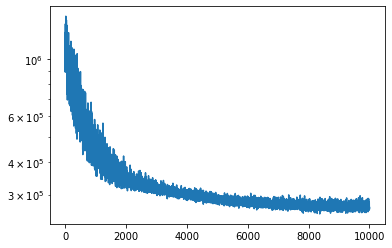
[17]:
plt.semilogy(posterior_pyro.loss_history)
[17]:
[<matplotlib.lines.Line2D at 0x7ff1559eda58>]
You can fit with the numpyro backend.
[12]:
%%time
from xidplus.numpyro_fit import SPIRE
fit_numpyro=SPIRE.all_bands([prior250,prior350,prior500])
CPU times: user 1min 2s, sys: 788 ms, total: 1min 3s
Wall time: 34.7 s
[13]:
posterior_numpyro=xidplus.posterior_numpyro(fit_numpyro,[prior250,prior350,prior500])
xidplus.save([prior250,prior350,prior500],posterior_numpyro,'test_numpyro')
Number of divergences: 0
[14]:
prior250.bkg
[14]:
(-5.0, 5)
CPU times: user 9min 17s, sys: 4.08 s, total: 9min 21s Wall time: 3min 33s
CPU times: user 59.6 s, sys: 511 ms, total: 1min Wall time: 27.3 s
[ ]: