XID+ Example Output Analysis

(This is based on a Jupyter notebook, available in the XID+ package and can be interactively run and edited)

This notebook provides some example code for basic analysis of the XID+ outputs, including:

1. Loading up output

2. Creating Posterior replicated maps and animations

3. Creating marginalised posterior plots

4. Creating Bayesian p-value maps

Import required modules

import pylab as plt
%matplotlib inline


import numpy as np
import xidplus
from xidplus import moc_routines
output_folder='./'

/Users/pdh21/anaconda3/envs/xidplus/lib/python3.6/site-packages/dask/config.py:168: YAMLLoadWarning: calling yaml.load() without Loader=... is deprecated, as the default Loader is unsafe. Please read https://msg.pyyaml.org/load for full details.
  data = yaml.load(f.read()) or {}
WARNING: AstropyDeprecationWarning: block_reduce was moved to the astropy.nddata.blocks module.  Please update your import statement. [astropy.nddata.utils]

Load up posterior output from XID+

priors,posterior=xidplus.load('test.pkl')

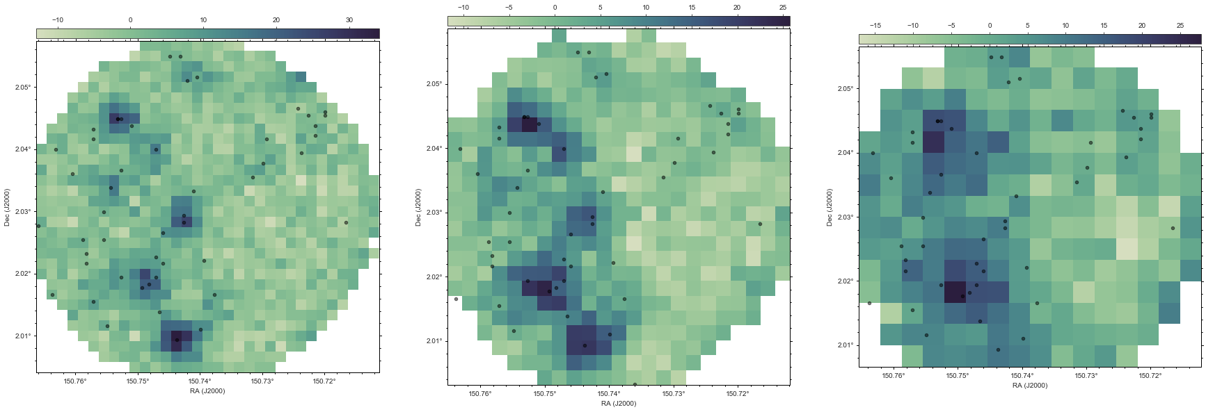
In order to compare how good our fit is, its often useful to look at original map. There is a routine within XID+ that makes the original fits map from the data stored within the prior class. Lets use that to make the SPIRE maps for the region we have fit.

Now lets use the Seaborn plotting package and APLpy package to view those maps, plotting the sources we have fit on top of those maps.

figs,fig=xidplus.plot_map(priors)

Posterior replicated data

We can use each sample we have from the posterior, and use it to make a replicated map, including simulating the instrumental noise, and the estimated confusion noise. You can think of these maps as all the possible maps that are allowed by the data.

NOTE: You will require the FFmpeg library installed to run the movie

xidplus.replicated_map_movie(priors,posterior,50)

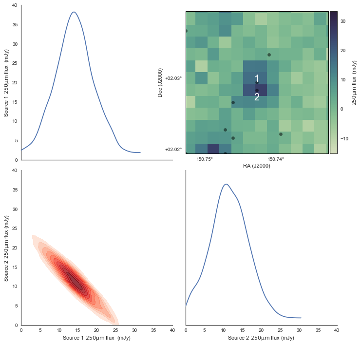
Joint Posterior Analysis of sources

#Select source you want to plot joint distribution
s1=2
s2=18

Sources 2 and 18 are close together, lets look at their joint posterior probabiity distribution. The code below is an example of how you can plot the joint posterior probability density function for the \(250 \mathrm{\mu m}\) flux, and an inset of the real map.

import aplpy
import seaborn as sns
sns.set(color_codes=True)
import pandas as pd
sns.set_style("white")
import xidplus.posterior_maps as postmaps



labels=[r'Source 1 $250\mathrm{\mu m}$ flux  (mJy)',r'Source 2 $250\mathrm{\mu m}$ flux (mJy)']
df = pd.DataFrame(posterior.samples['src_f'][:,0,[s1,s2]],columns=labels)
g = sns.PairGrid(df,size=5)
g.map_diag(sns.kdeplot,c='Red')
g.map_lower(sns.kdeplot, cmap="Reds",alpha=0.8,n_levels=10,normed=True, shade=True,shade_lowest=False)
g.set(ylim=(0,40))
g.set(xlim=(0,40))

g.axes[0,1].spines['bottom'].set_color('white')
g.axes[0,1].spines['left'].set_color('white')
cmap=sns.cubehelix_palette(8, start=.5, rot=-.75,as_cmap=True)

real_250 = aplpy.FITSFigure(postmaps.make_fits_image(priors[0],priors[0].sim)[1],figure=g.fig,subplot=(2,2,2))
real_250.show_colorscale(cmap=cmap)

real_250.show_markers(priors[0].sra, priors[0].sdec, edgecolor='black', facecolor='black',
                marker='o', s=40, alpha=0.5)
real_250.recenter(priors[0].sra[s1], priors[0].sdec[s1], radius=0.01)

real_250.add_label(priors[0].sra[s1], priors[0].sdec[s1]+0.0005, 1, relative=False,size=20,color='white')
real_250.add_label(priors[0].sra[s2], priors[0].sdec[s2]-0.0010, 2, relative=False,size=20,color='white')
real_250.tick_labels.set_xformat('dd.dd')
real_250.tick_labels.set_yformat('dd.dd')


real_250.add_colorbar(axis_label_text=r'$250\mathrm{\mu m}$ flux  (mJy)')

INFO: Auto-setting vmin to -1.522e+01 [aplpy.core]
INFO: Auto-setting vmax to  3.332e+01 [aplpy.core]

Posterior Predictive checking and Bayesian P-value maps

When examining goodness of fits, the typical method is to look at the residuals. i.e. \(\frac{data - model}{\sigma}\). Because we have distribution of \(y^{rep}\), we can do this in a more probabilisitic way using posterior predictive checks. For more information on posterior predictive checks, Gelman et al. 1996 is a good starting point.

For our case, the best way to carry out posterior predictive checks is to think about one pixel. We can look at where the real flux value for our pixel is in relation to the distribution from \(y^{rep}\).

from xidplus import posterior_maps as postmaps

rep_maps=postmaps.replicated_maps(priors,posterior)

import matplotlib as mpl
sns.set_style("white")

fig=plt.figure(figsize=(10,5))


# This is  the colormap I'd like to use.
cm = sns.diverging_palette(220, 20, as_cmap=True)

# Get the histogramp
Y,X = np.histogram(rep_maps[0][20,:], 25, normed=1)
#C = [cm(((x-X.min())/x_span)) for x in X]
C = [cm(((((x-np.mean(rep_maps[0][20,:]))/np.std(rep_maps[0][20,:]))+6)/12.0)) for x in X]


plt.bar(X[:-1],Y,color=C,width=X[1]-X[0])
plt.xlabel('Pixel Flux mJy')
plt.ylabel('p(pixel flux)')
plt.axvline(3.9, linestyle='--')
plt.axvline(-10.1,linestyle=':')
plt.annotate('flux in map that \n model cannot explain',xy=(4, 0.01),  xycoords='data',
            xytext=(4, 0.1), textcoords='data',rotation='vertical',size='large')
plt.annotate('too much flux in model \n compared to map',xy=(-10, 0.01),  xycoords='data',
            xytext=(-10, 0.1), textcoords='data',rotation='vertical',size='large')

#ax1 = fig.add_axes([0.05, 0.80, 0.9, 0.15])
ax1 = fig.add_axes([0.82, 0.15, 0.02, 0.7])

norm = mpl.colors.Normalize(vmin=-6, vmax=6)
cb1 = mpl.colorbar.ColorbarBase(ax1, cmap=cm,
                                norm=norm,
                                orientation='vertical')
cb1.set_label('$\sigma$')

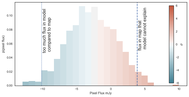
We can calculate fraction of \(y^{rep}\) samples above and below real map value. This is often referred to as the Bayesian p-value and is telling us the probability of drawing the real pixel value, from our model which has been inferred on the data. This is tells us if the model is inconsistent with the data, given the uncertianties in parameters and data.

• \(\sim 0.5\) means our model is consistent with the data

• 0.99 or 0.01 means model is missing something.

We can convert this to a typical ‘\(\sigma\)’ level and create map versions of these Bayesian p-values:

figs, fig=xidplus.plot_Bayes_pval_map(priors, posterior)

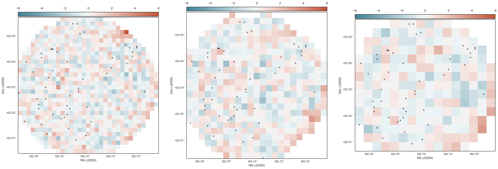
Red indicates the flux value in the real map is higher than our model thinks is possible. This could be indicating there is a source there that is not in our model. Blue indicates the flux in the real map is lower than in our model. This is either indicating a very low density region or that too much flux has been assigned to one of the sources.

Creating Catalogues

We can also create catalogues from the posterior probability density function

import xidplus.catalogue as cat

SPIRE_cat=cat.create_SPIRE_cat(posterior,priors[0],priors[1],priors[2])
SPIRE_cat.writeto('test.fits',overwrite=True)

Check table

Lets read in table with Astropy table

from astropy.table import Table

catalogue=Table.read('test.fits')

catalogue

<Table length=51>

HELP_ID	RA	Dec	F_SPIRE_250	FErr_SPIRE_250_u	FErr_SPIRE_250_l	F_SPIRE_350	FErr_SPIRE_350_u	FErr_SPIRE_350_l	F_SPIRE_500	FErr_SPIRE_500_u	FErr_SPIRE_500_l	Bkg_SPIRE_250	Bkg_SPIRE_350	Bkg_SPIRE_500	Sig_conf_SPIRE_250	Sig_conf_SPIRE_350	Sig_conf_SPIRE_500	Rhat_SPIRE_250	Rhat_SPIRE_350	Rhat_SPIRE_500	n_eff_SPIRE_250	n_eff_SPIRE_500	n_eff_SPIRE_350	Pval_res_250	Pval_res_350	Pval_res_500
	degrees	degrees	mJy	mJy	mJy	mJy	mJy	mJy	mJy	mJy	mJy	mJy/Beam	mJy/Beam	mJy/Beam	mJy/Beam	mJy/Beam	mJy/Beam
str27	float64	float64	float32	float32	float32	float32	float32	float32	float32	float32	float32	float32	float32	float32	float32	float32	float32	float32	float32	float32	float32	float32	float32	float32	float32	float32
1891	150.74711462	2.01937229149	3.7484	7.66319	1.18164	2.14374	4.78448	0.654144	3.95658	8.78007	1.13176	-2.55132	-4.50904	-6.23681	1.57567	1.54154	2.35809	1.00125	0.999651	0.999694	2000.0	2000.0	2000.0	0.0	0.001	0.0
1896	150.74655644	2.01381734435	4.60005	6.3697	2.84267	3.65866	5.48689	1.85056	1.92826	4.57817	0.519253	-2.55132	-4.50904	-6.23681	1.57567	1.54154	2.35809	1.00153	0.999281	1.00056	2000.0	2000.0	2000.0	0.0	0.003	0.0
2640	150.742672167	2.02937330604	13.9984	18.8843	9.17463	12.8981	15.4871	9.41806	1.86951	4.1993	0.517889	-2.55132	-4.50904	-6.23681	1.57567	1.54154	2.35809	1.00192	1.00116	1.00028	2000.0	2000.0	2000.0	0.0	0.008	0.0
5128	150.752680282	2.03659114242	3.17935	5.00112	1.51538	1.17502	2.5795	0.316155	4.84374	8.41198	1.72842	-2.55132	-4.50904	-6.23681	1.57567	1.54154	2.35809	0.999281	0.999725	0.999016	2000.0	2000.0	2000.0	0.0	0.017	0.001
5129	150.741006288	2.0332625701	4.14086	5.90487	2.33828	1.57266	3.09327	0.515144	2.12692	4.43263	0.572698	-2.55132	-4.50904	-6.23681	1.57567	1.54154	2.35809	0.999627	0.999396	0.999493	2000.0	2000.0	2000.0	0.0	0.018	0.0
5130	150.747123319	2.03992641714	15.163	16.7734	13.5599	18.3508	19.8903	16.8378	14.386	17.3602	11.346	-2.55132	-4.50904	-6.23681	1.57567	1.54154	2.35809	0.998979	0.998597	0.999077	2000.0	2000.0	2000.0	0.0	0.003	0.001
5159	150.754346603	2.03381290524	15.0139	16.8077	13.0577	7.17588	9.16244	4.82038	4.09872	7.76803	1.15535	-2.55132	-4.50904	-6.23681	1.57567	1.54154	2.35809	0.99918	1.00112	0.999327	2000.0	2000.0	2000.0	0.002	0.004	0.001
6067	150.755456605	2.02992385524	2.4755	4.13946	1.0596	5.07732	7.13054	3.02158	2.407	5.26434	0.697328	-2.55132	-4.50904	-6.23681	1.57567	1.54154	2.35809	1.00153	0.999871	0.999267	2000.0	2000.0	2000.0	0.002	0.023	0.002
6728	150.731557942	2.03548824889	2.27546	4.03699	0.814594	1.28256	2.65632	0.377102	1.25702	2.82928	0.311752	-2.55132	-4.50904	-6.23681	1.57567	1.54154	2.35809	0.999194	0.999004	0.999294	2000.0	2000.0	2000.0	0.001	0.0	0.002
...	...	...	...	...	...	...	...	...	...	...	...	...	...	...	...	...	...	...	...	...	...	...	...	...	...	...
54557	150.747116031	2.02270538967	4.16608	6.52053	2.01011	1.80936	3.88562	0.481275	3.85372	8.23103	1.19911	-2.55132	-4.50904	-6.23681	1.57567	1.54154	2.35809	0.999127	0.998905	0.999505	2000.0	2000.0	2000.0	0.0	0.003	0.0
56696	150.721556173	2.04382481093	0.88412	2.1644	0.240798	0.949373	2.36094	0.255432	1.20004	3.06691	0.313454	-2.55132	-4.50904	-6.23681	1.57567	1.54154	2.35809	0.999351	0.998961	1.00171	2000.0	2000.0	2000.0	0.014	0.002	0.008
56700	150.729337091	2.04159980217	1.48247	2.86367	0.449076	1.04582	2.22337	0.322739	1.39198	3.18743	0.412141	-2.55132	-4.50904	-6.23681	1.57567	1.54154	2.35809	0.999942	0.999822	0.99837	2000.0	2000.0	2000.0	0.001	0.0	0.004
57200	150.740458126	2.05159489041	10.474	12.744	7.8894	4.53638	6.91396	2.20241	2.68414	5.65835	0.824703	-2.55132	-4.50904	-6.23681	1.57567	1.54154	2.35809	0.998646	0.99865	0.999078	2000.0	2000.0	2000.0	0.0	0.001	0.005
58792	150.739334129	2.02215285778	1.53584	2.8906	0.536787	1.04091	2.18379	0.311871	1.33951	2.95336	0.337598	-2.55132	-4.50904	-6.23681	1.57567	1.54154	2.35809	0.999491	1.00085	0.999512	2000.0	2000.0	2000.0	0.0	0.002	0.0
62679	150.751015847	2.04381351831	2.44807	4.68218	0.755575	2.66707	5.36711	0.964311	3.18924	7.19739	0.878154	-2.55132	-4.50904	-6.23681	1.57567	1.54154	2.35809	0.999891	0.999694	1.00034	2000.0	2000.0	2000.0	0.0	0.0	0.004
62696	150.716547293	2.02827210175	0.900113	1.87745	0.273319	1.05167	2.08977	0.323288	2.6556	4.82945	0.958473	-2.55132	-4.50904	-6.23681	1.57567	1.54154	2.35809	0.998641	1.00014	0.998887	2000.0	2000.0	2000.0	0.001	0.068	0.226
64788	150.757117895	2.01547979941	7.4053	8.99943	5.69952	6.23498	8.09541	4.30285	1.50978	3.65069	0.413473	-2.55132	-4.50904	-6.23681	1.57567	1.54154	2.35809	0.999124	0.99898	0.999234	2000.0	2000.0	2000.0	0.0	0.003	0.004
64789	150.722668543	2.04549095568	0.693414	1.73135	0.171959	1.00955	2.43527	0.254088	1.50451	3.61353	0.414402	-2.55132	-4.50904	-6.23681	1.57567	1.54154	2.35809	0.999581	1.00064	1.00024	2000.0	2000.0	2000.0	0.319	0.001	0.002
64790	150.746006008	2.02659443544	3.66645	5.70863	1.70092	9.75185	11.836	7.74227	2.95004	5.88184	0.874799	-2.55132	-4.50904	-6.23681	1.57567	1.54154	2.35809	1.00089	1.00012	0.999632	2000.0	2000.0	2000.0	0.0	0.004	0.0